Number Theoretic Transform - A Gentle Introduction: Part II

“A Monet painting of convolution” by DALL-E 2.
The Number Theoretic Transform
Previously, we took a look at the problem of polynomial multiplication. Specifically, we saw that we can view polynomial multiplications as a form of convolution. To make things easier to compute, we often define a polynomial modulus, making it into a ring. The modulus defining the ring in our context is often special, making the convolution either circular or negative wrapped.
At the end of the last post, we saw a naive approach at speeding up computation of convolutions - by converting the polynomials into evaluation form so convolution is as simple as coordinate-wise multiplication. We end up on the problem of the conversion between coefficient form and evaluation form which is expensive and becomes the new bottleneck.
In this post, we will now look at an efficient solution: Number Theoretic Transform, or NTT for short.
Images used in this post are sourced from this great survey on NTT - Number Theoretic Transform and Its Applications in Lattice-based Cryptosystems: A Survey.
NTT: A Primer
So, what is NTT? If we look at Wikipedia, NTT is a particular flavor of Discrete Fourier Transform (DFT) over a finite field. I could write another 2 to 3 pages worth of content to dive into Fourier Transform, its continuous and discrete variants, and the Fast Fourier Transform (FFT) algorithm. But I think it might not be the best use of our time in this particular post about NTT. Therefore, if you want to know more about how DFT works, I’d highly recommend checking out this amazing tutorial by 3Blue1Brown, and this follow-up video by Reducible.
Instead, we will take a Computer Science or programming perspective to look at what NTT is. Given a length-$d$ vector $\mathbf{a} = {a_0, a_1, \dots, a_{d-1}}$, a carefully-selected prime modulus finite field $\mathbb{Z}_q$, and a primitive $d$-th root of unity $\omega_d$ (meaning that $\omega_d^d \equiv 1 (\text{mod } q)$, and that the smallest positive $i$ such that $\omega_d^i$ satisfies this relation is $d$), NTT defines the following transformation:
$$ \begin{align*} \hat{\mathbf{a}} &= NTT(\mathbf{a}) \\ &= \left(\hat{a}_j = \sum_{i=0}^{d-1} a_i \omega_d^{ij} \right)_{j \in [0, \dots, d-1]} \end{align*} $$
Essentially, for a length-$d$ vector, NTT transforms that vector into another length-$d$ vector, but computes some kind of summation of all terms in the original vector mixed with the root of unity $\omega_d$.
Some Observations
Although this NTT expression looks intimidating at the first glance, we can actually find very interesting similarities between this and something we have seen before.
Let’s compute the first element of $NTT(\mathbf{a})$:
$$ \begin{align*} \hat{\mathbf{a}}_0 &= \sum_{i=0}^{d-1} a_i \omega_d^{0 \cdot i}\\ &= \sum_{i=0}^{d-1} a_i (\omega_d^0)^i \end{align*} $$
Similarly, let’s compute the second element:
$$ \begin{align*} \hat{\mathbf{a}}_1 &= \sum_{i=0}^{d-1} a_i \omega_d^{1 \cdot i}\\ &= \sum_{i=0}^{d-1} a_i (\omega_d)^i \end{align*} $$
If we read through our previous blog post in this series, we can immediately notice that these expression are no different from evaluating the polynomial $a(x)$ at points $\omega_d^0$ and $\omega_d^1$. We can easily see that the other entries of $\hat{\mathbf{a}}$ correspond to evaluation of $a(x)$ at the remaining powers $\omega_d^j$.
Since $\omega_d$ is a primitive $d$-th root of unity, we know that all its powers within $[0, d-1]$ are distinct. The proof is also simple: assume the powers of $\omega_d$ are not unique, then we will find two different powers $\omega_d^i = \omega_d^j$ where $i \ne j, 0 \le i < j \le d-1$. If this is true, we can derive $\omega_d^{j-i} = \frac{\omega_d^j}{\omega_d^i} = 1$. However, this clearly contradicts with the primitive root requirement, where the smallest positive power of $\omega_d$ that equals to 1 is $d$, hence such collision cannot exist. Therefore, when we interpret NTT as polynomial evaluation at powers of $\omega_d$, we know that all the evaluation points are distinct!
What about its inverse?
We know that NTT is no different from evaluating a degree-$(d-1)$ polynomial at $d$ distinct points. In the previous post, we saw the technique of polynomial interpolation that will recover the original polynomial from the distinct $d$ evaluations. Similarly, there is an inverse transformation iNTT that takes us back from the NTT (evaluation) form to the regular coefficient form.
The Inverse Number Theoretic Transform is defined quite beautifully:
$$ \begin{align*} \mathbf{a} &= iNTT(\hat{\mathbf{a}}) \\ &= \left(a_j = d^{-1} \sum_{i=0}^{d-1} \hat{a}_i \omega_d^{-ij} \right)_{j \in [0, \dots, d-1]} \end{align*} $$
Basically, we take the inverse of the original $d$-th root of unity $\omega_d^{-1}$, and apply the exact same NTT algorithm on the NTT form, plus a minor tweak where we need to apply a scaler $d^{-1}$ to properly scale the coefficients down.
For now, we are not going to be super concerned about what Inverse NTT does. We just assume this subroutine magically works and converts the NTT form back to the coefficient form.
# We fix a small modulus for testing purposes
MODULUS = 17
GEN = 13
# 13 is a primitive 4-th root of unity of modulus 17.
# Therefore, we will be working with polynomials with length 4 (degree 3).
assert pow(GEN, 4, MODULUS) == 1

def naive_ntt(a, gen=GEN, modulus=MODULUS):
  deg_d = len(a)
  out = [0] * deg_d

  # We precompute omega terms to avoid recomputing them in the next block.
  omegas = [0] * deg_d
  omegas[0] = 1
  for i in range(1, len(omegas)):
    omegas[i] = omegas[i-1] * gen % modulus

  for i in range(deg_d):
    for j in range(deg_d):
      # Perform the NTT summation: \sum a_j * omega_d^{ij}
      out[i] = (out[i] + a[j] * omegas[i * j % deg_d]) % modulus

  return out

def naive_intt(a, gen=GEN, modulus=MODULUS):
  deg_d = len(a)
  out = [0] * deg_d

  omegas = [0] * deg_d
  omegas[0] = 1
  for i in range(1, len(omegas)):
    omegas[i] = omegas[i-1] * pow(gen, -1, modulus) % modulus

  for i in range(deg_d):
    for j in range(deg_d):
      out[i] = (out[i] + a[j] * omegas[i * j % deg_d]) % modulus

  # Scale it down before returning.
  scaler = pow(deg_d, -1, modulus)
  return [i * scaler % modulus for i in out]

a = [1, 2, 3, 4]
a_ntt = naive_ntt(a)
a_intt = naive_intt(a_ntt)
print(a)
print(a_ntt)
print(a_intt)
assert a == a_intt
[1, 2, 3, 4]
[10, 6, 15, 7]
[1, 2, 3, 4]
Speeding up, yet again…
Now we have seen the naive implementation of NTT and Inverse NTT, something has caught our attention: the code for NTT is again some double iterative summation over all coefficients, which immediately screams $O(d^2)$ complexity. Our sole intention of going to the NTT domain is to avoid the $O(d^2)$ cost of convolution, therefore, we have to figure out ways to speed up this routine, or we will get no benefit at all.
Fortunately, this is where the magic of Fast Fourier Transform (FFT) starts to shine. We are not going to go in details of what FFT is, but let’s pay attention to the following expansion and grouping of the NTT algorithm. To make things more readable, we use $NTT_{\omega_k}$ to represent NTT algorithm for dimension-$k$ vector using primitive $k$-th root of unity.
$$ \begin{align*} NTT_{\omega_d}(\mathbf{a})_j &= \sum_{i=0}^{d-1} a_i \omega_d^{ij}\\ &= \sum_{i=0}^{\frac{d}{2}-1} a_{2i} \omega_d^{2ij} + \sum_{i=0}^{\frac{d}{2}-1} a_{2i+1} \omega_d^{(2i+1)j}\\ &= \sum_{i=0}^{\frac{d}{2}-1} a_{2i} (\omega_d^2)^{ij} + \omega_d^j \sum_{i=0}^{\frac{d}{2}-1} a_{2i+1} (\omega_d^2)^{ij}\\ &= NTT_{\omega_{d/2}}(\mathbf{a}^\text{even})_j + \omega_d^j NTT_{\omega_{d/2}}(\mathbf{a}^\text{odd})_j \end{align*} $$
Essentially, what the expansion above does is to separate out the even-indexed coefficients in $\mathbf{a}$ from the odd ones, and the expression becomes two shorter NTT subroutines that uses the primitive $(d/2)$-th root of unity. We have thus found ourselves a recurrence relation!
To make things nice, we will always work with some degree $d$ that’s a power of 2. Therefore we are sure that $d$ will be splittable all the way till 1. And at the bottom of the recursion, NTT of some length-1 vector is just itself - think of evaluating a degree-0 polynomial, which is just the constant coefficient.
Looking at the recurrence relation, at each layer, we are doing the job of one addition plus one multiplication by a constant $\omega_d^j$, therefore it’s $O(d)$ work to perform coordinate-wise addition and scaling. We break the task into 2 smaller tasks, each with half the size, therefore going down $O(\log{d})$ levels. This will get us $O(d \log{d})$ total runtime complexity, which is a great improvement from $O(d^2).$
However, the expression above only applies for $0 \le j < \frac{d}{2}$, as once $j$ exceeds the boundary, the behavior becomes undefined (you cannot get the $(d/2+1)$-th index of a NTT that’s only $d/2$ long). But what happens for points beyond $\frac{d}{2}$? Let’s give it a try: if we look closely at the original expression evaluated at point $j’ = \frac{d}{2} + j$:
$$ \begin{align*} NTT_{\omega_d}(\mathbf{a})_{\frac{d}{2} + j} &= \sum_{i=0}^{d-1} a_i \omega_d^{i(\frac{d}{2} + j)}\\ &= \sum_{i=0}^{d-1} a_i (\omega_d^{\frac{d}{2} + j})^i\\ &= \sum_{i=0}^{d-1} a_i (\omega_d^{\frac{d}{2}} \omega_d^j)^i\\ &= \sum_{i=0}^{d-1} a_i (-\omega_d^j)^i\\ &= \sum_{i=0}^{d-1} (-1)^i a_i \omega_d^{ij}\\ &= \sum_{i=0}^{\frac{d}{2}-1} a_{2i} \omega_d^{2ij} - \sum_{i=0}^{\frac{d}{2}-1} a_{2i+1} \omega_d^{(2i+1)j}\\ &= NTT_{\omega_{d/2}}(\mathbf{a}^\text{even})_j - \omega_d^j NTT_{\omega_{d/2}}(\mathbf{a}^\text{odd})_j \end{align*} $$
One crucial observation here is that since $w_d^d \equiv 1$, we know that $w_d^\frac{d}{2} \equiv -1 (\text{mod } q)$. This is because the two roots of 1 are itself and -1, and since $w_d^\frac{d}{2} \ne w_d^d$ due to the definition of the primitive root of unity, it has to be the other root that corresponds to -1. Then we can replace all the occurence of $\omega_d^\frac{d}{2}$ with simply -1, and the NTT at point $\frac{d}{2} + j$ magically equals to the NTT at point $j$ with the symbol before the odd term flipped.
With this new finding in mind, here is the plan to implement the recursive NTT:
- Define the base case (NTT of a single element is itself).
- Break the input vector into even and odd parts, and recursively call NTT on them with the $\omega$ term squared.
- For $0 \le j < \frac{d}{2}$, fill the output array with $NTT_{\omega_{d/2}}(\mathbf{a_j}^\text{even}) + \omega_d^j NTT_{\omega_{d/2}}(\mathbf{a_j}^\text{odd})$.
- For $\frac{d}{2} \le j < d$, fill the output array with $NTT_{\omega_{d/2}}(\mathbf{a_j}^\text{even}) - \omega_d^j NTT_{\omega_{d/2}}(\mathbf{a_j}^\text{odd})$. Note that step 3 and 4 can be combined in a single loop to avoid recomputing the two terms.
Now, let’s implement the improved subroutines to supercharge NTT. This recursive algorithm is also called a Radix-2 Cooley-Tukey NTT algorithm, named after Cooley and Tukey who (re)discovered the FFT algorithm in 1965.
def cooley_tukey_ntt(a, gen=GEN, modulus=MODULUS):
  # Base case: the NTT of a single element is itself.
  if len(a) == 1:
    return a[:]

  # Precompute the omega terms.
  omegas = [0] * len(a)
  omegas[0] = 1
  for i in range(1, len(omegas)):
    omegas[i] = omegas[i-1] * gen % modulus

  # Recursive step.
  # We break the original vector a into even part and odd part.
  # Then we perform NTT on both parts, using omega^2 as the generator.
  even = cooley_tukey_ntt([a[i] for i in range(0, len(a), 2)], pow(gen, 2, modulus), modulus)
  odd = cooley_tukey_ntt([a[i] for i in range(1, len(a), 2)], pow(gen, 2, modulus), modulus)

  # Piece the results together.
  out = [0] * len(a)
  for k in range(len(a)//2):
    p = even[k]
    q = (omegas[k] * odd[k]) % modulus
    out[k] = (p + q) % modulus
    out[k + len(a)//2] = (p - q) % modulus
  return out

a_ct_ntt = cooley_tukey_ntt(a)
print(a_ct_ntt)
assert a_ct_ntt == a_ntt
[10, 6, 15, 7]
Cooley-Tukey butterfly
After completing the recursive version of the NTT algorithm, we ask ourselves again: can we do better?
The answer is always: Yes! In fact, although recursion is a nice way to express the recurrence relation, it isn’t the most efficient way, considering the number of nested function calls will cost us in the call stack and the recomputation of certain values. Therefore, can we come up with an iterative version of NTT?
In order to do so, we are going to follow the instructions given by Chapter 30.3 in Introduction to Algorithms. First, let’s try to expand the recursive call hierarchy of an example input of length-8.
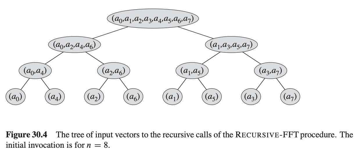
NTT recursive expansion.
From the expansion, we can see at the bottom, pairs of two elements are grouped together: $(a_0, a_4), (a_2, a_6), (a_1, a_5), (a_3, a_7)$. Interestingly, the difference between the indices of the two elements are all 4, half of the total length.
Walking upwards the tree, every parent node combines the elements inside the leaf nodes in two different ways: $even \pm \omega^j odd$, thus generating a result vector that has twice the size as its leaves.
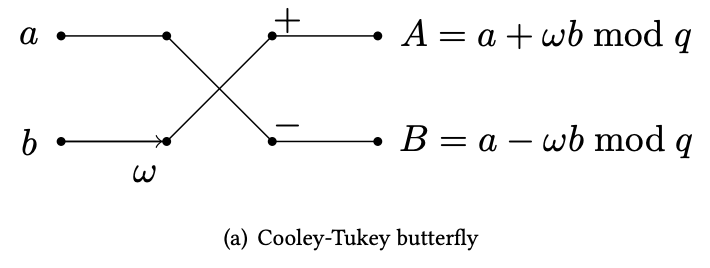
Cooley-Tukey butterfly.
This kind of structure can be depicted with a diagram that shows how the two parts of the input (even and odd) can be combined together and form two outputs. Given the shape of the data flow, this operation is commonly referred as the butterfly operation. In particular, what we have here is the Cooley-Tukey butterfly.
Now, we have two ideas:
Recursion is really an iterative grouping of elements in a particular order.
The “grouping” operation is the Cooley-Tukey butterfly operation.
Combining both ideas, we can sketch out a “circuit” design for the NTT procedure:
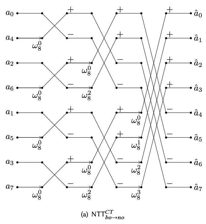
NTT Cooley-Tukey butterfly network circuit.
And the iterative version of the NTT algorithm can be described by interpreting the circuit diagram from left to right:
- Reorganize the input in this special interleaved order.
- Apply the first level CT butterfly operation with $\omega_2^j$ (2-th root of unity as the recursive step deals with array of length 2).
- Apply the second level CT butterfly operation on the previous result with the 4-th root of unity $\omega_4^j$. Note that this is equivalent to the previous step, except we doubled the stride of the butterfly operation.
- Iteratively apply the CT butterfly operation until the end. In the last layer, the stride length should be half of the total vector length (4 in our case).
Now, this procedure requires this weird shuffling of the input to match the base level of the recursion. But interestingly, this shuffle order is actually just the bit-reverse of the index. Why? Because the last bit of a number decides whether it’s even or odd. And in the recursive step, we separate elements in the array based on their parity - or the last bit. And at the next step, we look at their second last bit and group them up accordingly.
def brv(x, n):
  """ Reverses a n-bit number """
  return int(''.join(reversed(bin(x)[2:].zfill(n))), 2)

print(list(range(8)))
print(list([brv(i, 3) for i in range(8)]))
[0, 1, 2, 3, 4, 5, 6, 7]
[0, 4, 2, 6, 1, 5, 3, 7]
Another interesting approach to understand this is to think that we are sorting the indices of the array by looking at the least significant bit first, then progress all the way to the most significant bit - hence the sorted order is just bit-reverse of the original order.
With the bit-reversal helper in place, we can move onto implementing the iterative NTT.
import math

def ntt_iter(a, gen=GEN, modulus=MODULUS):
  deg_d = len(a)

  # Start with stride = 1.
  stride = 1

  # Shuffle the input array in bit-reversal order.
  nbits = int(math.log2(deg_d))
  res = [a[brv(i, nbits)] for i in range(deg_d)]

  # Pre-compute the generators used in different stages of the recursion.
  gens = [pow(gen, pow(2, i), modulus) for i in range(nbits)]
  # The first layer uses the lowest (2nd) root of unity, hence the last one.
  gen_ptr = len(gens) - 1

  # Iterate until the last layer.
  while stride < deg_d:
    # For each stride, iterate over all N//(stride*2) slices.
    for start in range(0, deg_d, stride * 2):
      # For each pair of the CT butterfly operation.
      for i in range(start, start + stride):
        # Compute the omega multiplier. Here j = i - start.
        zp = pow(gens[gen_ptr], i - start, modulus)

        # Cooley-Tukey butterfly.
        a = res[i]
        b = res[i+stride]
        res[i] = (a + zp * b) % modulus
        res[i+stride] = (a - zp * b) % modulus

    # Grow the stride.
    stride <<= 1
    # Move to the next root of unity.
    gen_ptr -= 1

  return res

a_ntt_iter = ntt_iter(a)
print(a_ntt_iter)
assert a_ntt_iter == a_ct_ntt
[10, 6, 15, 7]
Gentleman-Sande butterfly
Now we have mastered the Cooley-Tukey butterfly network. The inverse transformation uses a circuit gadget that reverses (or unmixes) the result from a CT butterfly. This gadget is called the Gentleman-Sande butterfly as shown in the diagram below.
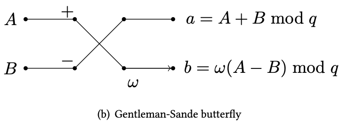
Gentleman-Sande butterfly.
The inverse transform is exactly reversing the entire CT butterfly network, and thus forming the GS butterfly network.
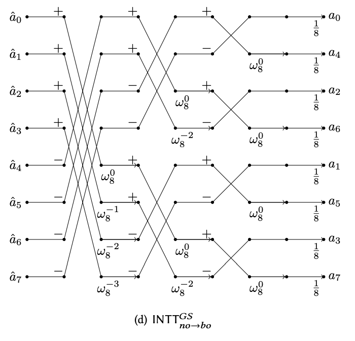
iNTT Gentleman-Sande butterfly network circuit.
Essentially, for the iNTT circuit, we just perform the Gentleman-Sande butterfly operation to undo the Cooley-Tukey butterfly operation at the layers from right to left in the perspective of the NTT circuit.
We will code up the iNTT algorithm below. Notice the very subtle differences of this compared to the algorithm above. In fact, because they are so similar, often when implemented in hardware, they can share most of the circuitry, plus/minus some tweaks to adjust the omega values and the strides.
def intt_iter(a, gen=GEN, modulus=MODULUS):
  deg_d = len(a)

  # Start with stride = N/2.
  stride = deg_d // 2

  # Shuffle the input array in bit-reversal order.
  nbits = int(math.log2(deg_d))
  res = a[:]

  # Pre-compute the inverse generators used in different stages of the recursion.
  gen = pow(gen, -1, modulus)
  gens = [pow(gen, pow(2, i), modulus) for i in range(nbits)]
  # The first layer uses the highest (d-th) root of unity, hence the first one.
  gen_ptr = 0

  # Iterate until the last layer.
  while stride > 0:
    # For each stride, iterate over all N//(stride*2) slices.
    for start in range(0, deg_d, stride * 2):
      # For each pair of the CT butterfly operation.
      for i in range(start, start + stride):
        # Compute the omega multiplier. Here j = i - start.
        zp = pow(gens[gen_ptr], i - start, modulus)

        # Gentleman-Sande butterfly.
        a = res[i]
        b = res[i+stride]
        res[i] = (a + b) % modulus
        res[i+stride] = ((a - b) * zp) % modulus

    # Grow the stride.
    stride >>= 1
    # Move to the next root of unity.
    gen_ptr += 1

  # Scale it down before returning.
  scaler = pow(deg_d, -1, modulus)

  # Reverse shuffle and return.
  return [(res[brv(i, nbits)] * scaler) % modulus for i in range(deg_d)]

a_intt_iter = intt_iter(a_ntt_iter)
print(a_intt_iter)
assert a_intt_iter == a
[1, 2, 3, 4]
And finally… We are here, with an efficient NTT/iNTT algorithm that takes a polynomial into the NTT domain and roundtrips it back.
If you are able to follow this post until this point, big congrats to you! As this is already a big achievement ;)
Have we forgotten the rings?
Now that we have defined the efficient subroutines that performs NTT and iNTT, the next question naturally rises: how do we use this latest and greatest piece of work to perform the calculation we really care about: circular convolution and negative wrapped convolution of two polynomials $P, Q$?
Fortunately, we can quickly use the formula we derived at the end of the last post to achieve this. Here we use $\mathbf{p}, \mathbf{q}$ to represent the vector of coefficients in polynomial $P, Q$ that have size $d$.
Extend the vectors $\mathbf{p}, \mathbf{q}$ to be length $2d$ by filling the latter extended part to be zero. $\mathbf{p}' = [p_0, \dots, p_{d-1}, 0, \dots, 0], \mathbf{q}' = [q_0, \dots, q_{d-1}, 0, \dots, 0]$
Perform $NTT$ on the extended vector $\mathbf{p}', \mathbf{q}'$ and obtain $\hat{\mathbf{p}'}, \hat{\mathbf{q}'}$.
Multiply $\hat{\mathbf{p}'}, \hat{\mathbf{q}'}$ component wise.
Apply $iNTT$ to get the result: $\mathbf{r} = iNTT(\hat{\mathbf{p}'} \otimes \hat{\mathbf{q}')}$, where $\otimes$ represents coordinate-wise multiplication.
Intepret the result $\mathbf{r}$ as a degree $2d - 2$ polynomial, and reduce it by the polynomial modulus $x^d \pm 1$. The coefficients of the reduced polynomial $\mathbf{r}_\text{red}$ is the final result.
# First, we introduce some reference code we borrowed from the previous post for testing correctness.
# BEGIN: REFERENCE
def mul_poly_naive_q_cc(a, b, q, d):
  tmp = [0] * (d * 2 - 1) # intermediate polynomial has degree 2d-2

  # schoolbook multiplication
  for i in range(len(a)):
    # perform a_i * b
    for j in range(len(b)):
      tmp[i + j] = (tmp[i + j] + a[i] * b[j]) % q

  # take polynomial modulo x^d - 1
  for i in range(d, len(tmp)):
    tmp[i - d] = (tmp[i - d] + tmp[i]) % q
    tmp[i] = 0

  return tmp[:d]

def mul_poly_naive_q_nwc(a, b, q, d):
  tmp = [0] * (d * 2 - 1) # intermediate polynomial has degree 2d-2

  # schoolbook multiplication
  for i in range(len(a)):
    # perform a_i * b
    for j in range(len(b)):
      tmp[i + j] = (tmp[i + j] + a[i] * b[j]) % q

  # take polynomial modulo x^d + 1
  for i in range(d, len(tmp)):
    tmp[i - d] = (tmp[i - d] - tmp[i]) % q
    tmp[i] = 0

  return tmp[:d]
# END: REFERENCE
# We need a new generator since we are working with vectors of length 8 instead of 4.
MODULUS = 17
GEN = 8 # 8 has order 8 in mod 17

def ntt_mul_cc_attempt(p, q, gen=GEN, modulus=MODULUS):
  deg_d = len(p)

  # Extend the vectors to length-2d
  pp = p + [0] * deg_d
  qq = q + [0] * deg_d

  # Perform NTT.
  pp_ntt = ntt_iter(pp, gen, modulus)
  qq_ntt = ntt_iter(qq, gen, modulus)

  # Component wise multiplication.
  rr_ntt = [(i * j) % modulus for i, j in zip(pp_ntt, qq_ntt)]

  # Convert back to coefficient form.
  rr = intt_iter(rr_ntt, gen, modulus)

  # take polynomial modulo x^d - 1
  for i in range(deg_d, len(rr)):
    rr[i - deg_d] = (rr[i - deg_d] + rr[i]) % modulus
    rr[i] = 0

  return rr[:deg_d]

def ntt_mul_nwc_attempt(p, q, gen=GEN, modulus=MODULUS):
  deg_d = len(p)

  # Extend the vectors to length-2d
  pp = p + [0] * deg_d
  qq = q + [0] * deg_d

  # Perform NTT.
  pp_ntt = ntt_iter(pp, gen, modulus)
  qq_ntt = ntt_iter(qq, gen, modulus)

  # Component wise multiplication.
  rr_ntt = [(i * j) % modulus for i, j in zip(pp_ntt, qq_ntt)]

  # Convert back to coefficient form.
  rr = intt_iter(rr_ntt, gen, modulus)

  # take polynomial modulo x^d + 1
  for i in range(deg_d, len(rr)):
    rr[i - deg_d] = (rr[i - deg_d] - rr[i]) % modulus
    rr[i] = 0

  return rr[:deg_d]

p = [1, 2, 3, 4]
q = [1, 3, 5, 7]

pq_cc_attempt = ntt_mul_cc_attempt(p, q)
print(pq_cc_attempt)
assert pq_cc_attempt == mul_poly_naive_q_cc(p, q, MODULUS, len(p))

pq_nwc_attempt = ntt_mul_nwc_attempt(p, q)
print(pq_nwc_attempt)
assert pq_nwc_attempt == mul_poly_naive_q_nwc(p, q, MODULUS, len(p))
[8, 12, 8, 13]
[11, 15, 3, 13]
And… it works!
However, although it’s working great, the additional reduction operation always feels a bit cumbersome. It looks a bit out-of-place and inelegant. What if we can somehow do the reduction also as part of the NTT?
Let’s expand on how we actually perform reduction operation first. Consider the evaluation form of polynomial $P$ before and after reduction.
$$ \begin{align*} P_\text{red}(x) &= (P \text{ mod } \phi)(x)\\ &= (P - k \phi)(x)\\ &= \sum_i p_i x^i - k \phi_i x^i\\ &= (\sum_i p_i x^i) - k (\sum_i \phi_i x^i)\\ &= P(x) - k\phi(x) \end{align*} $$
Here, $k$ is some constant value which makes sure the order of $P_\text{red}$ is smaller than the order of $\phi$. We can see that reducing a polynomial by another polynomial is really subtracting copies of the modulus from the original polynomial.
Here is an interesting idea: if the point $x$ where we evaluate happens to be a root of $\phi$, i.e., $\phi(x) = 0$, then in the evaluation form the reduction has no effect! This means, even without an explicit reduction step, the resulting polynomial when we convert back to the coefficient form is “automagically” reduced.
This is nice, but how do we apply this idea to the entire NTT procedure? In two steps:
- We find $d$ distinct roots of the reduction polynomial $x^d \pm 1$.
- We evaluate the degree-$(d-1)$ polynomial at those $d$ distinct points.
- Profit. I mean really now we don’t need the reduction step, and the result will be auto-reduced.
This is good news. There is even a better news: since the coefficients will be automatically reduced and thus have order less than $d$, we don’t need to evaluate $2d$ points anymore. Instead, we can always work with $d$ points as they can uniquely define any order $d-1$ polynomial.
Finding roots for circular convolution
Next, we can plug in the reduction polynomial $x^d - 1$ for the case of circular convolution, and see whether we can make this auto-reduction magic happen.
Right now, all we know is that $d$ is a power of two, so it can be divided many times before it reaches 1. Before we introduce any tricks, let’s try to expand the terms and look for the root ourselves.
$$ \begin{align*} x^d - 1 &= (x^\frac{d}{2} - 1) (x^\frac{d}{2} + 1)\\ &= (x^\frac{d}{4} - 1) (x^\frac{d}{4} + 1) (x^\frac{d}{2} + 1)\\ &= (x^\frac{d}{8} - 1) (x^\frac{d}{8} + 1) (x^\frac{d}{4} + 1) (x^\frac{d}{2} + 1)\\ &= (x - 1) (x + 1) (x^2 + 1) (x^4 + 1) \dots (x^\frac{d}{2} + 1) \\ \end{align*} $$
Till this point, we have already fully expanded the leftmost term down to $x-1$ and cannot reduce any further. The remaining terms are higher order addition terms and it looks like we cannot make any progress. However, since we know that $\omega_d^\frac{d}{2} \equiv -1$, we can rewrite the term $x^\frac{d}{2} + 1 \rightarrow x^\frac{d}{2} - \omega_d^\frac{d}{2}$, which allows us to split further.
By recursively doing the reduction and replacement of positive terms with $-\omega_d^i$ powers, we are able to split the polynomial and derive the following tree structure.
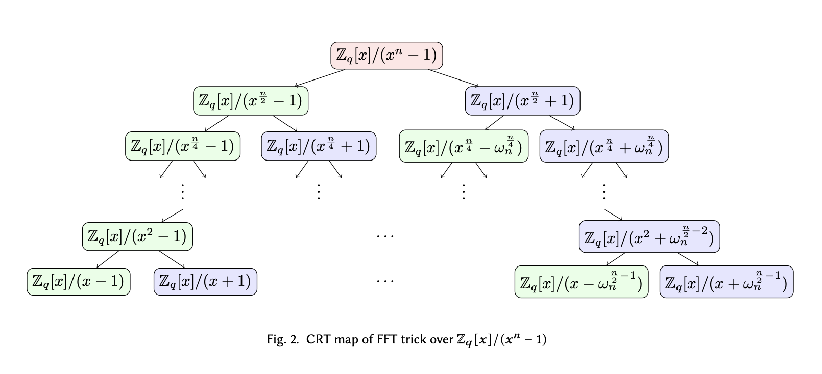
Recursively factor circular convolution modulus.
On the leaf layer of the tree, we essentially factored the polynomial modulus $x^d$ (written as $x^n$ in the diagram) into $d$ degree-1 terms. Each term thus represents a root to the reduction polynomial, which is the point we want NTT to evaluate at, to avoid doing additional reduction step.
Note that on the diagram above, it says something about “CRT map”. Don’t worry about what it is for now, as we will discuss more in detail about the similarities between CRT mapping, polynomial reduction and polynomial evaluation in the next post.
But now we have the comprehensive list of roots that we want to evaluate at:
$$ [1, -1, \omega_d, -\omega_d, \omega_d^2, -\omega_d^2, \dots, \omega_d^{\frac{d}{2} - 1}, -\omega_d^{\frac{d}{2} - 1}] $$
Since we know that $\omega_d^\frac{d}{2} = -1$, and obviously $\omega_d^0 = 1$, we can rewrite the list as:
$$ [\omega_d^0, \omega_d^1, \omega_d^2, \dots, \omega_d^\frac{d}{2}, \omega_d^{\frac{d}{2} + 1}, \dots, \omega_d^{d - 1}] $$
Hence, this is the same as the entire set generated by the $d$-th primitive root of unity, which is what our existing NTT routing has been doing all the time.
TL;DR: No change is needed! By applying the plain NTT operation, we already obtain evaluations of the polynomial at the roots of the polynomial modulus, so we can just do the component-wise multiplication in the regular length-$d$ NTT form, and convert it back.
Here is the implementation:
# Now we can use the original generator again, because we don't need to work in dimension-2d.
MODULUS = 17
GEN = 13

def ntt_mul_cc_no_red(p, q, gen=GEN, modulus=MODULUS):
  # Perform NTT.
  p_ntt = ntt_iter(p, gen, modulus)
  q_ntt = ntt_iter(q, gen, modulus)

  # Component wise multiplication.
  r_ntt = [(i * j) % modulus for i, j in zip(p_ntt, q_ntt)]

  # Convert back to coefficient form.
  rr = intt_iter(r_ntt, gen, modulus)
  return rr

pq_cc_no_red = ntt_mul_cc_no_red(p, q)
print(pq_cc_no_red)
assert pq_cc_no_red == mul_poly_naive_q_cc(p, q, MODULUS, len(p))
[8, 12, 8, 13]
Finding roots for negative wrapped convolution
Now let’s try the same trick on the polynomial modulus $x^d + 1$ for the NWC case. We apply a slightly different replacement trick:
$$ \begin{align*} x^d + 1 \equiv x^d - (-1) &\equiv x^d - \omega_d^\frac{d}{2}\\ &= (x^\frac{d}{2} - \omega_d^\frac{d}{4})(x^\frac{d}{2} + \omega_d^\frac{d}{4})\\ &= (x^\frac{d}{4} - \omega_d^\frac{d}{8})(x^\frac{d}{4} + \omega_d^\frac{d}{8})(x^\frac{d}{2} + \omega_d^\frac{d}{4})\\ &= \dots \end{align*} $$
We omit the full reduction step and only show the front. However, one can quickly notice a discrepancy of this reduction tree versus the previous one: When expanding $x^d - 1$, the degree of $x$ and $\omega_d$ are always the same - always $x^\frac{d}{2^k} \pm \omega_d^\frac{d}{2^k}$. However, when we are expanding $x^d + 1$, the degree of $\omega_d$ is always half of that of $x$.
Since we know that $d$ can only be divided $log_2(d)$ number of times, it means, when at the second layer from the bottom, the $\omega_d$ term would already have an odd degree - like $x^2 \pm \omega_d$. Even by subsituting it with it’s negation form, the degree is still odd and it doesn’t allow us to split further. If we cannot split the polynomial to a multiple of degree-1 terms, then we cannot directly infer the roots from the expression itself.
Looks like we’ve hit a dead end.
But let’s not give up just now. There are actually two options to move forward:
Work with this reduction and try to see if there are some properties we can use to help with NWC.
Introduce some more structure and assumptions to this problem to make the last split feasible.
We are going to look at Approach 2 this time. We will try to cover Approach 1 in the next post.
How can we further split the term $x^2 - \omega_d$? Obviously, if we can find the square root of $\omega_d$ in the underlying field $\mathbb{Z}_q$, then we solve the problem.
Going along that thought, let’s assume there exists a $2d$-th primitive root of unity $\psi_{2d}$ such that $\psi_{2d}^2 = \omega_d$, then we can do the last split as $x^2 - \omega_d \rightarrow (x + \psi_{2d}) (x - \psi_{2d})$.
Using $\psi_{2d}$ as the new order-$2d$ generator, we can rewrite the entire reduction tree as:
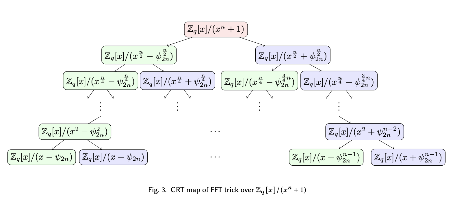
Recursively factor negatively-wrapped convolution modulus.
On the bottom layer, we see the roots are essentially power of $\psi_{2n}$ that splits the odd powers of $\omega_d$.
Therefore, the $d$ odd powers $\{psi_{2d}^{2i+1}\}_{i \in [d]}$ can uniquely define the evaluation points we need to make NWC happen without additional reduction. The even powers of $\psi_{2d}$ are also powers of $\omega_d$, so they aren’t present in the last layer.
Now let’s formulate the NTT algorithm that uses odd powers of $\psi_{2d}$:
$$ \begin{align*} NTT_\psi(\mathbf{a})_j &= \sum_{i=0}^{d-1} a_i \psi_{2d}^{i \cdot (2j+1)}\\ &= \sum_{i=0}^{d-1} a_i \psi_{2d}^{2ij} \psi_{2d}^i\\ &= \sum_{i=0}^{d-1} a_i \omega_d^{ij} \psi_{2d}^i\\ &= NTT_\omega([\psi_{2d}^0 a_0, \psi_{2d}^1 a_1, \dots, \psi_{2d}^{d-1} a_{d-1}])_j \end{align*} $$
We can see that, evaluating the polynomial at the odd powers of $\psi_{2d}$ is equivalent of multiplying the coefficients of the polynomial with powers of $\psi_{2d}$ beforehand, and then feed into the regular length-$d$ NTT algorithm that uses $\omega_d$.
Conversly, the inverse transformation would be first inverting via the regular NTT, and then apply the inverse of $\psi_{2d}^i$ to each coefficient correspondingly.
At last, let’s try to implement this new version of the NTT:
# We need the 2d-th root of unity. d=4.
MODULUS = 17
GEN_4 = 13 # d-th root
GEN_8 = 8 # 2d-th root
GEN_8_INV = pow(GEN_8, -1, MODULUS)

GEN_8_POW = [pow(GEN_8, i, MODULUS) for i in range(8)]
GEN_8_INV_POW = [pow(GEN_8_INV, i, MODULUS) for i in range(8)]

def ntt_mul_nwc_no_red(p, q, gen=GEN_4, modulus=MODULUS):
  # Preprocess P and Q.
  pp = [(p[i] * GEN_8_POW[i]) % MODULUS for i in range(len(p))]
  qq = [(q[i] * GEN_8_POW[i]) % MODULUS for i in range(len(q))]

  # Perform NTT.
  p_ntt = ntt_iter(pp, gen, modulus)
  q_ntt = ntt_iter(qq, gen, modulus)

  # Component wise multiplication.
  r_ntt = [(i * j) % modulus for i, j in zip(p_ntt, q_ntt)]

  # Convert back to coefficient form.
  rr = intt_iter(r_ntt, gen, modulus)
  return [(rr[i] * GEN_8_INV_POW[i]) % MODULUS for i in range(len(rr))]

pq_nwc_no_red = ntt_mul_nwc_no_red(p, q)
print(pq_nwc_no_red)
assert pq_nwc_no_red == mul_poly_naive_q_nwc(p, q, MODULUS, len(p))
[11, 15, 3, 13]
Field Size Matters
In order for this approach to work, a crucial requirement is that there has to exist such $\psi_{2d}$ in the underlying finite field $\mathbb{Z}_q$. This immediately means that even if we are not doing length-$2d$ NTTs, to multiply degree $d$ polynomials without reduction, the underlying field has to be large enough such that we could do length-$2d$ NTTs.
We can safely ignore this quirk for now. But this will soon come haunt us when we look into real life Lattice-based Cryptographic Schemes, such as Kyber. But no worries for now, we will get you ready for that in the next post ;)
Conclusion
First of all, congratulations to you if you have made to this part of the blog post! I’m glad that you have finally understood the inner workings (and beauty) of NTT!
To conclude, we have covered the following in this blog post:
- What NTT really is - it’s summation form, as well as understanding it as evaluating and interpolating polynomials.
- How to efficiently run NTT - using Cooley-Tukey and Gentleman-Sande butterfly network, as well as doing them iteratively via a bit-reversal shuffle.
- Lastly, how to use NTT to perform convolution in cyclic and negative wrapped scenarios. More importantly, how to save the extra reduction step by picking the right generators (in many places, $\omega_d$ and $\psi_{2d}$ are also referred to as “twiddle factors”).
In our next post, we will dive into real life use cases of NTT, such as the CRYSTALS-Kyber cryptosystem that has been standardized by NIST as the next generation post-quantum key-encapsulation mechanism. We will also take a look at tips and tricks to make NTT run faster and with smaller footprints. See you all next time!